E127: Quadratic prime-run atlas (\(n^2 + a n + b\))
Tags: number-theory, quantitative-exploration, visualization, primes, optimization
See: Valid Tags.
Highlights
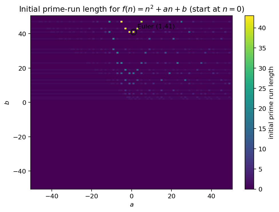
Heatmap of “how long primes last” for \(f(n)=n^2+an+b\) across a small (a,b) grid.
Euler’s \((a,b)=(1,41)\) appears as a visible peak, but it is not unique.
Turns a folklore fact into a reproducible, parameterized sweep with saved artifacts.
Goal
Explore how sensitive initial prime streaks are to the coefficients of a quadratic polynomial. We measure, for each (a,b), the largest \(L\) such that \(f(0),f(1),\dots,f(L-1)\) are all prime.
Background (quick refresher)
Research question
Within a bounded coefficient grid, which quadratic polynomials produce the longest initial prime runs, and where does Euler’s polynomial sit in that landscape?
Method
Sweep integers \(a\in[a_{\min},a_{\max}]\) and \(b\in[b_{\min},b_{\max}]\).
For each pair, evaluate \(f(n)\) for \(n=0..N\) and record the initial prime-run length.
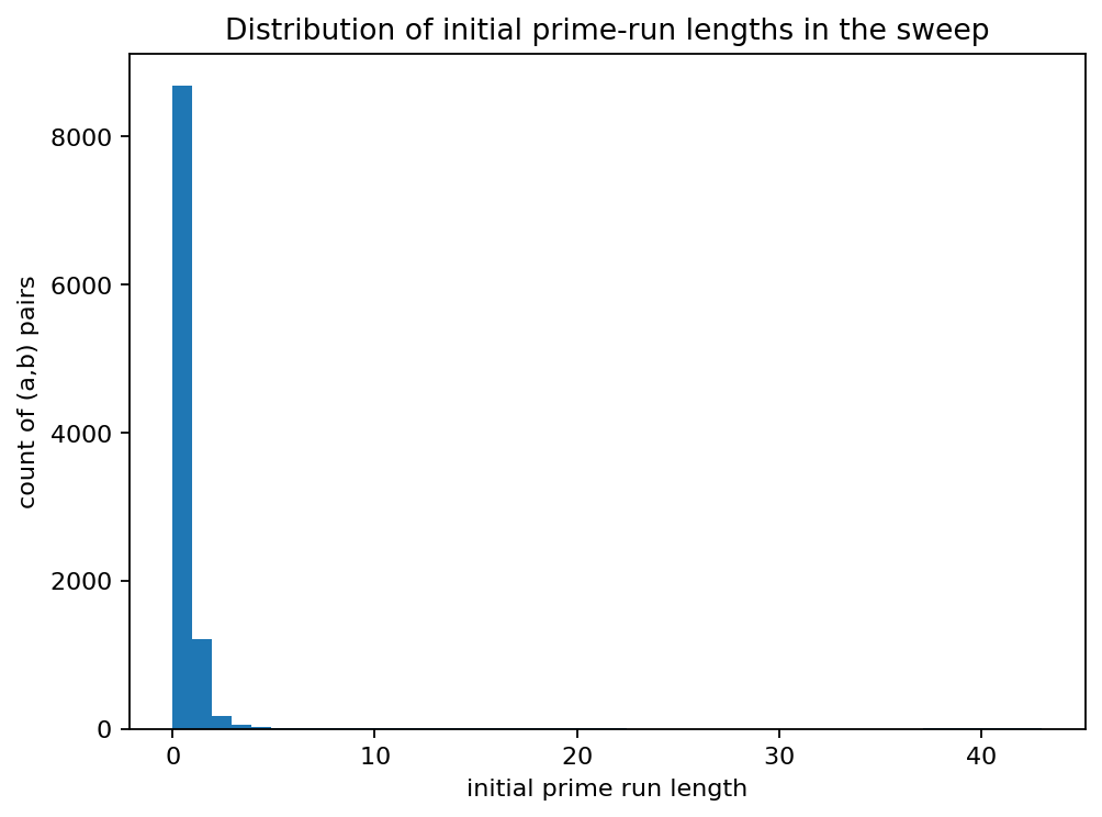
Visualize run length as a heatmap and summarize the top candidates in the report.
Plot axes and coordinate conventions
The heatmap uses a 2D grid over the integer coefficients \((a,b)\):
x-axis: the coefficient \(a\) (horizontal direction)
y-axis: the coefficient \(b\) (vertical direction)
If the sweep uses unit steps (the default), then each heatmap cell corresponds directly to an integer pair:
More generally, if the heatmap array is indexed by \((i,j)\) with \(i=0,\dots,n_a-1\) (columns) and \(j=0,\dots,n_b-1\) (rows), then the coefficients shown at that cell are:
- \[x = a = a_{\min} + i\,\Delta a\]
- \[y = b = b_{\min} + j\,\Delta b\]
For Matplotlib imshow, this is typically implemented via an extent so that tick labels match the coefficient values
(e.g. extent=(a_min-0.5, a_max+0.5, b_min-0.5, b_max+0.5) for unit steps). If you flip the image origin (origin="upper"),
the y-axis is inverted visually; in that case, interpret the y-axis tick labels accordingly.
How to run
make run EXP=e127
or:
uv run python -m mathxlab.experiments.e127
Outputs
This experiment follows the standard output contract:
out/e127/figures/— generated figures (PNG)out/e127/report.md— short narrative reportout/e127/params.json— run parameters (stable JSON)out/e127/logs/— run logs (created by the runner/Makefile)
Published run snapshot
If this experiment is included in the docs gallery, include the published snapshot (report + params).
Reproduce:
make run EXP=e127
Parameters
a range:
[-50, 50]b range:
[-50, 50]n_run_max:
80(test n=0..n_run_max)top_k:
12
Key observation
Initial prime streaks vary sharply across (a,b). A few islands can look remarkably prime-rich on small ranges, which explains why Euler’s famous polynomial stands out in short scans.
Euler point (a=1,b=41) in this grid: run length 40 (n=0..39).
Best run lengths in this sweep
run length |
a |
b |
polynomial |
|---|---|---|---|
43 |
-5 |
47 |
\(n^2 + -5n + 47\) |
42 |
-3 |
43 |
\(n^2 + -3n + 43\) |
41 |
-1 |
41 |
\(n^2 + -1n + 41\) |
40 |
1 |
41 |
\(n^2 + 1n + 41\) |
39 |
3 |
43 |
\(n^2 + 3n + 43\) |
38 |
5 |
47 |
\(n^2 + 5n + 47\) |
22 |
-11 |
47 |
\(n^2 + -11n + 47\) |
21 |
-9 |
37 |
\(n^2 + -9n + 37\) |
20 |
-7 |
29 |
\(n^2 + -7n + 29\) |
19 |
-5 |
23 |
\(n^2 + -5n + 23\) |
18 |
-3 |
19 |
\(n^2 + -3n + 19\) |
17 |
-1 |
17 |
\(n^2 + -1n + 17\) |
Outputs
figures/fig_01_run_length_heatmap.pngfigures/fig_02_run_length_histogram.pngparams.jsonreport.md
params.json (snapshot)
{
  "a_max": 50,
  "a_min": -50,
  "b_max": 50,
  "b_min": -50,
  "n_run_max": 80,
  "seed": 1,
  "top_k": 12
}