E003: Abundancy Index Landscape
Tags: number-theory, quantitative-exploration, visualization, numerics
See: Valid Tags.
Highlights
Compute \(\sigma(1..N)\) via a divisor-sum sieve.
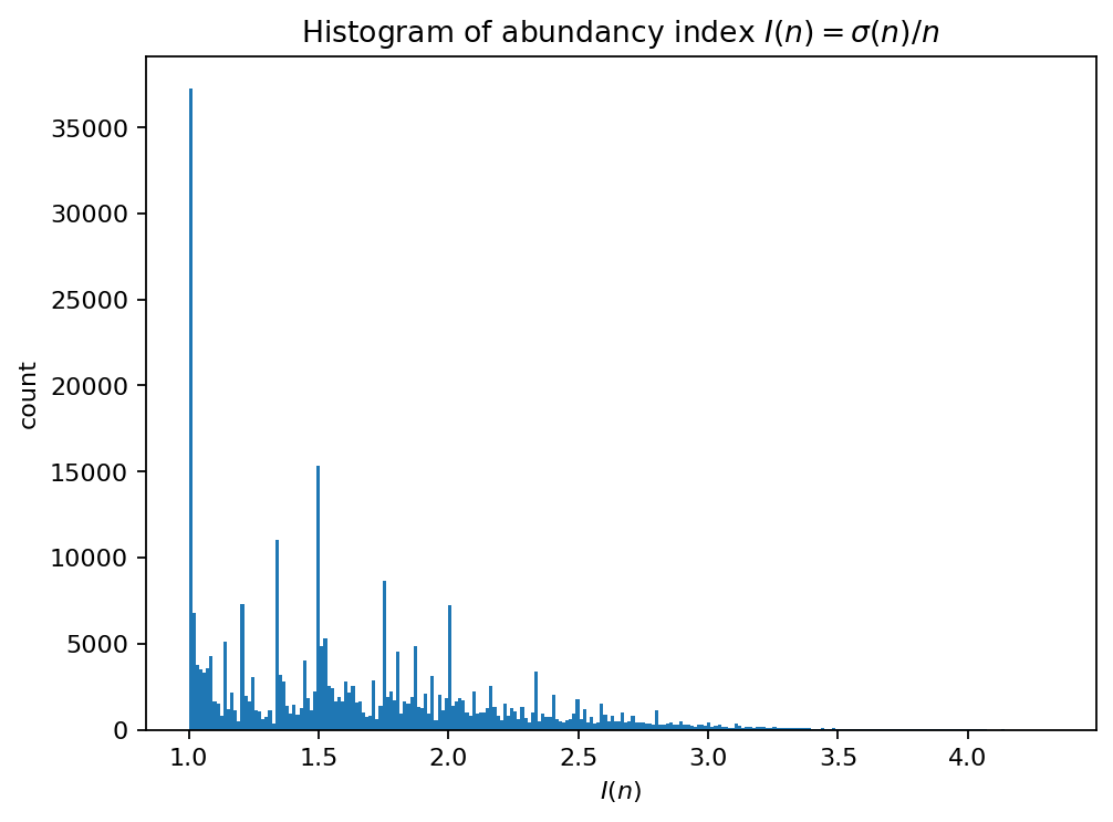
Visualize the distribution of \(I(n)=\sigma(n)/n\).
Highlight perfect numbers as the razor-thin level set \(I(n)=2\).
Goal
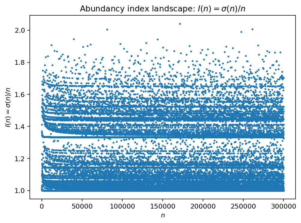
Visualize how rare perfect numbers are by plotting the distribution of the abundancy index
Research question
For a given bound \(N\):
What does the empirical distribution of \(I(n)\) look like?
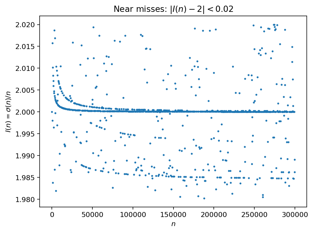
How frequently do we see values near \(2\)?
Where do the perfect numbers appear in the landscape?
Why this qualifies as a mathematical experiment
The divisor-sum function \(\sigma(n)\) is highly structured but “spiky” and hard to intuit symbolically. Computational sweeps reveal qualitative structure (clusters, gaps, tails) and put perfect numbers into context.
Experiment design
Method: compute \(\sigma(1)\), …, \(\sigma(N)\) via a divisor-sum sieve
Use the identity “each divisor contributes to its multiples”:
initialize an array
sigma[0..N]with zerosfor each
d = 1..N:add
dtosigma[k]for all multiplesk = d, 2d, 3d, ...
This runs in about \(O(N\log N)\) time and avoids per-number factorization.
Observables
\(I(n) = \sigma(n)/n\)
distance to perfection: \(|I(n)-2|\)
classification:
deficient: \(I(n)<2\)
perfect: \(I(n)=2\)
abundant: \(I(n)>2\)
Plots
histogram of \(I(n)\) (or of \(I(n)-1\))
scatter plot of \(n\) vs. \(I(n)\) (optionally with log-scale on \(n\))
highlight perfect numbers
How to run
make run EXP=e003
or:
uv run python -m mathxlab.experiments.e003
Notes / pitfalls
\(I(n)\) is rational. For classification, compare integers using \(\sigma(n)\) and \(2n\) rather than floats.
For plots, floats are fine, but compute the “perfect” condition as
sigma[n] == 2*n.Start with \(N \le 1\,000\,000\) to keep runtime and memory reasonable.
Extensions
Repeat for different ranges and overlay histograms.
Plot the top-\(k\) values of \(I(n)\) and compare to known extremal families.
Explore the “near misses” set (feeds directly into E006).
Published run snapshot
If this experiment is included in the docs gallery, include the published snapshot (report + params).
Reproduce:
make run EXP=e003
Parameters
N:
300000scatter stride:
10histogram bins:
250near band:
0.02
Outputs
figures/fig_01_hist_abundancy.pngfigures/fig_02_scatter_abundancy.pngfigures/fig_03_near_2.pngparams.json
Findings
Perfect numbers found (≤ N):
4
Notes
Compare perfection using integers: σ(n) == 2n.
For plotting, floats are acceptable, but classification should not depend on float rounding.
params.json (snapshot)
{
  "bins": 250,
  "n_max": 300000,
  "near_band": 0.02,
  "stride_scatter": 10
}
References
See References.