E019: Prime counting and a PNT baseline

Published run: \(\text{n}_{\max} = 200\,000\) and \(\pi(\text{n}_{\max}) = 17\,984\)

Published run: \(\text{n}_{\max} = 2\,000\,000\) and \(\pi(\text{n}_{\max}) = 148\,933\)

Published run: \(\text{n}_{\max} = 10\,000\,000\) and \(\pi(\text{n}_{\max}) = 664\,579\)

Published run: \(\text{n}_{\max} = 30\,000\,000\) and \(\pi(\text{n}_{\max}) = 1\,857\,859\)

Prime counts shown are \(\pi(\text{n}_{\max})\), i.e., the number of primes \(\le \text{n}_{\max}\). In this experiment we evaluate \(\pi(x)\) for all integers \(x\) with \(2 \le x \le \text{n}_{\max}\).

Tags: number-theory, quantitative-exploration, visualization
See: Valid Tags.

Highlights

• Visual sanity check for your prime pipeline: compute \(\pi(x)\) from a sieve mask and compare to a standard smooth baseline.

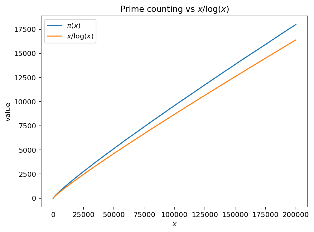
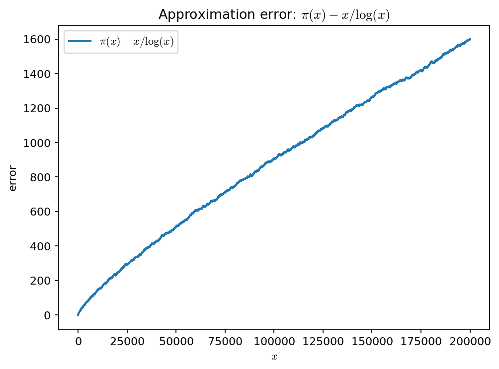
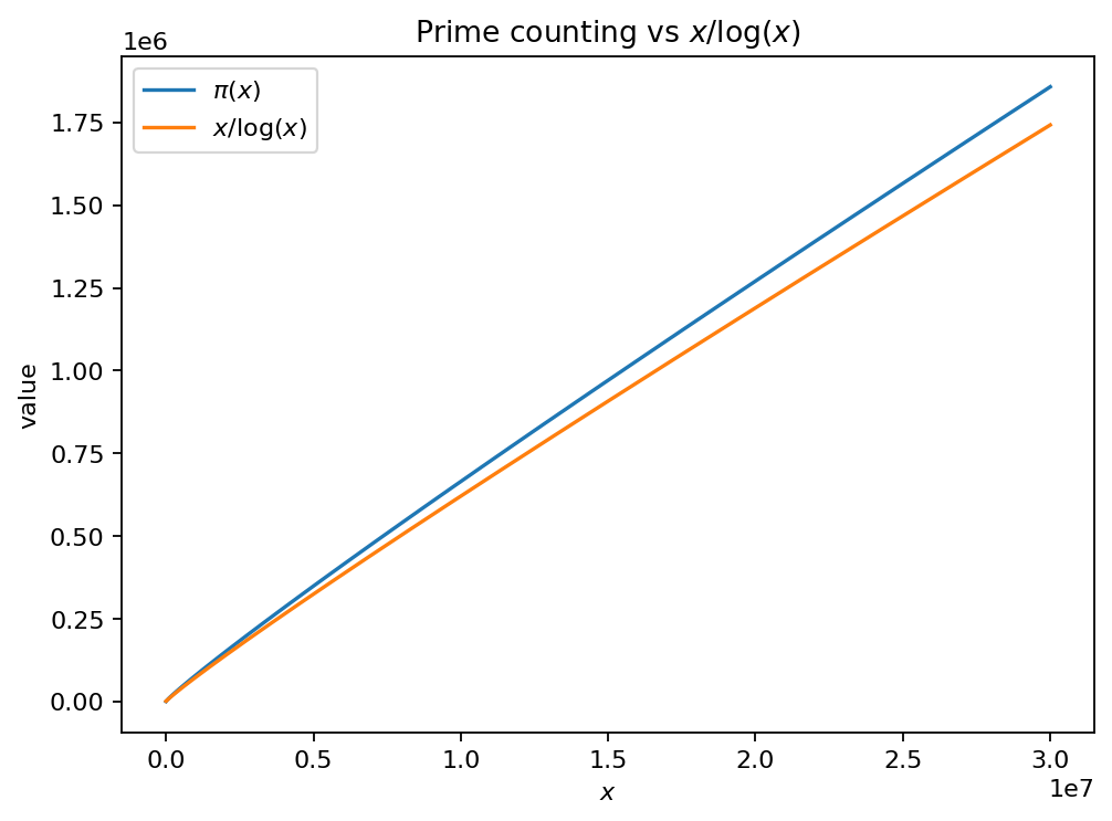
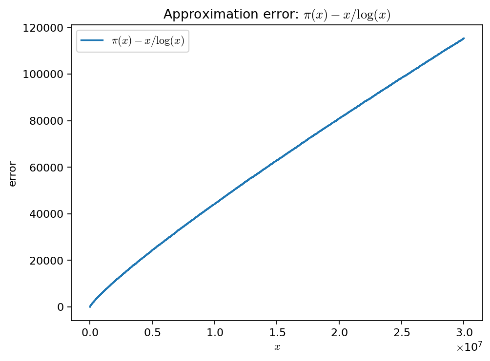
• Two complementary plots: \(\pi(x)\) vs. \(x/\log(x)\), and the finite-range error curve \(\pi(x) - x/\log(x)\).

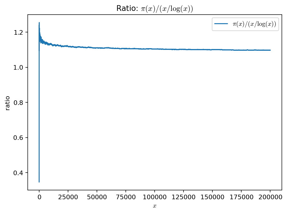
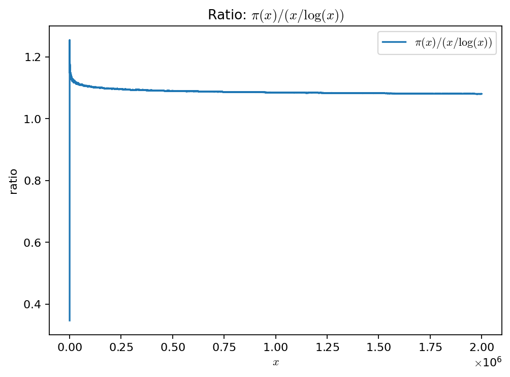
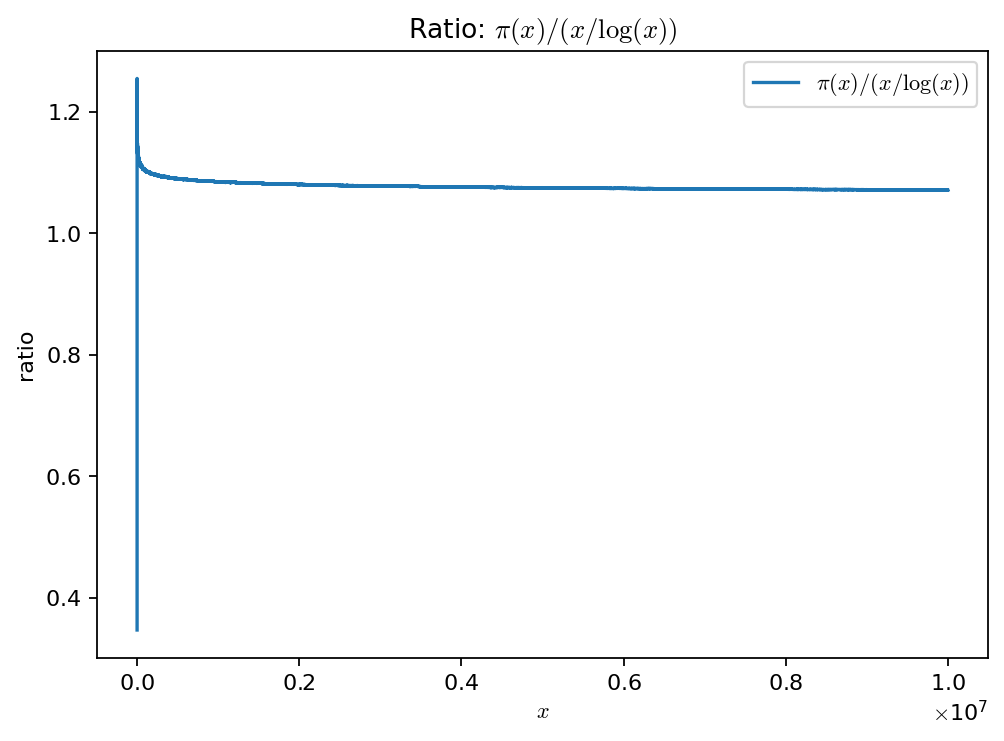
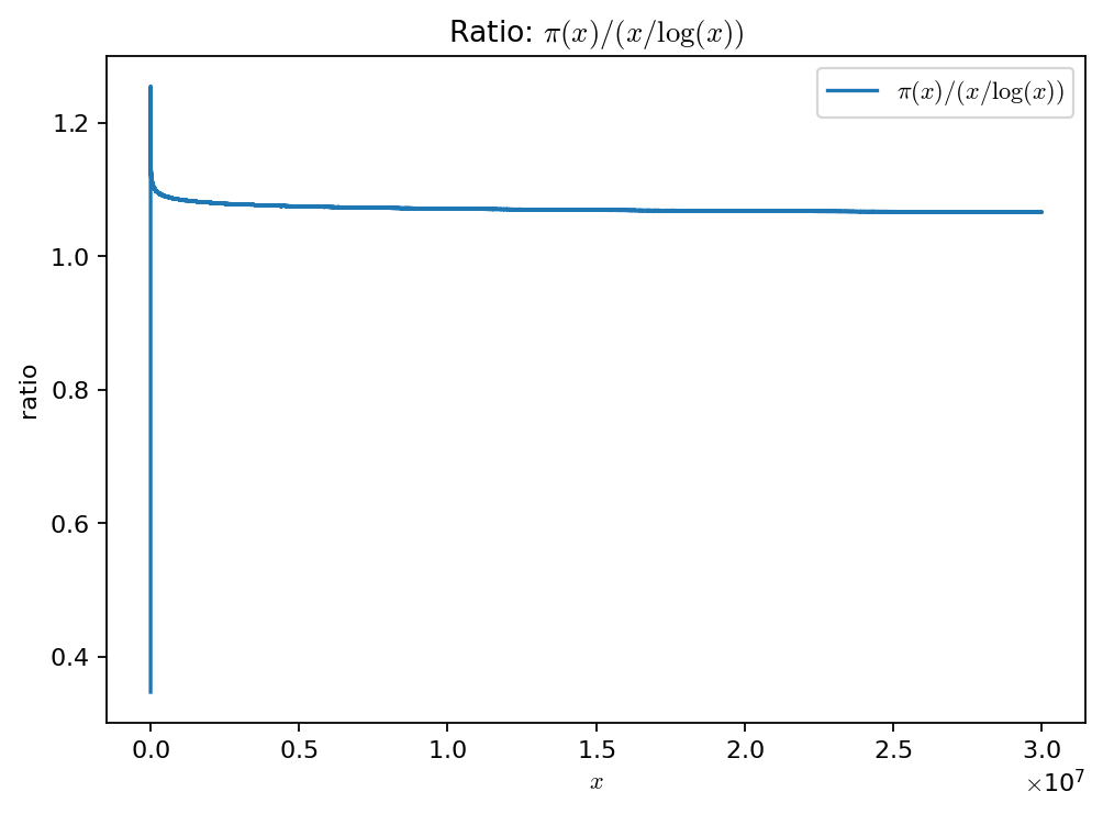
• Ratio plot: \(\pi(x) / (x/\log(x))\) makes relative deviation visible when the two curves nearly overlap.

• Writes reproducible artifacts (params.json, report.md, and figures) into out/e019/.

Goal

Visualize how well the Prime Number Theorem baseline \(x/\log(x)\) tracks the prime-counting function \(\pi(x)\) on a finite range and makes the approximation error visible.

Background (quick refresher)

Prime-counting function

The prime-counting function \(\pi(x)\) is the number of primes \(p\) with \(p \le x\).

The PNT baseline

The Prime Number Theorem (PNT) states that

\[ \pi(x) \sim \frac{x}{\log x} \quad \text{as } x \to \infty. \]

Here \(\log\) is the natural logarithm. The symbol “\(\sim\)” is asymptotic: it does not claim the two expressions are close for small or moderate \(x\).

Optional background pages

• Prime counting approximations: π(x), Li(x), and R(x)

• Prime counting: explicit bounds (not just asymptotics)

• Prime numbers refresher

Research question

On the finite range \(2 \le x \le \text{n}_{\max}\):

1. How close is \(x/\log(x)\) to \(\pi(x)\) as \(x\) grows?

2. What does the finite-range error \(\pi(x) - x/\log(x)\) look like (trend, scale, rough smoothness)?

Why this qualifies as a mathematical experiment

• Finite procedure: compute primes up to \(\text{n}_{\max}\), then compute the cumulative count \(\pi(x)\).

• Observable(s): the comparison curve \(\pi(x)\) vs. \(x/\log(x)\) and the finite-range error curve.

• Parameter space: \(\text{n}_{\max}\) (and, if you extend it, sampling choices such as linear vs. log-spaced grids).

• Outcome: figures plus a short report capturing the key observation and caveats.

• Reproducibility: outputs saved to out/e019/ with a parameter snapshot.

Experiment design

• Computation:

  • Build a prime mask for \(\{0,1,\dots,\text{n}_{\max}\}\) using a sieve.

  • Convert the mask to a cumulative array so that \(\pi(x)\) can be read off quickly.

  • For each integer \(x\) with \(2 \le x \le \text{n}_{\max}\), compute the baseline \(x/\log(x)\).

• Axes (what the plots mean):

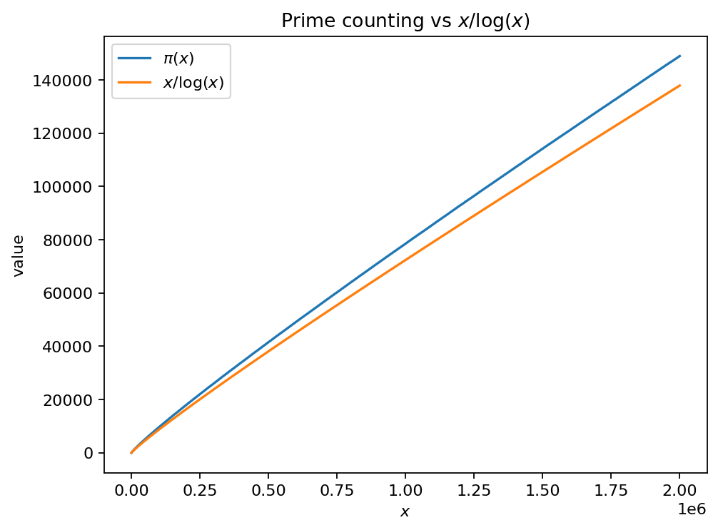
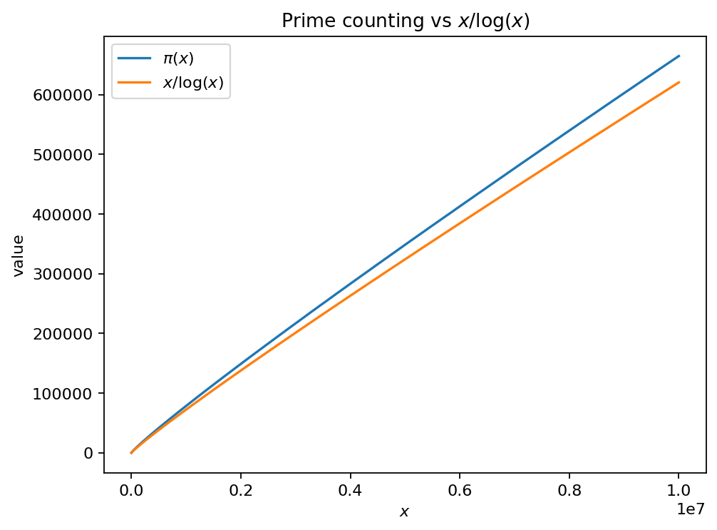
  • In the first plot, the horizontal axis is \(x\) and the vertical axis is a count: it shows \(\pi(x)\) and \(x/\log(x)\) for the same \(x\) values.

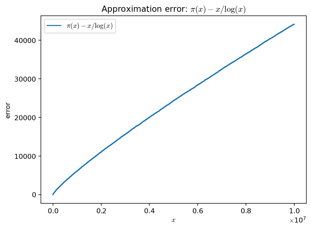
  • In the second plot, the horizontal axis is \(x\) and the vertical axis is the count difference \(\pi(x) - x/\log(x)\).

• Outputs (typical):

  • figures/fig_01_pi_vs_x_logx.png

  • figures/fig_02_pi_minus_x_logx.png

  • figures/fig_03_pi_over_x_logx_ratio.png

  • params.json

  • report.md

How to run

make run EXP=e019

Override the upper bound (computes primes up to \(\text{n}_{\max}\)):

make run EXP=e019 ARGS="--n-max 5000000"

Direct invocation (always works):

uv run --extra dev python -m mathxlab.experiments.e019 --out out/e019
# Override the upper bound:
uv run --extra dev python -m mathxlab.experiments.e019 --out out/e019 --n-max 5000000

Notes / pitfalls

• Finite-range behavior: the PNT statement is asymptotic; interpret these plots as “finite-range behavior”.

• Parameter exposure: use --n-max to change \(\text{n}_{\max}\); keep published snapshots consistent with params.json / report.md.

• Scale masking: on a linear axis, \(\pi(x)\) and \(x/\log(x)\) are close in relative terms, so runs with different \(\text{n}_{\max}\) can look very similar. Use the ratio plot \(\pi(x) / (x/\log(x))\) for a relative view.

• Log domain: avoid \(x=0\) or \(x=1\) because \(\log(x)\) is \(0\) or undefined there; we start at \(x=2\).

• Visual overclaims: a smooth-looking error curve does not imply a theorem about error terms.

Extensions

• Add a second baseline \(\mathrm{Li}(x)\) and compare \(\pi(x) - \mathrm{Li}(x)\).

• Add explicit bounds (Rosser–Schoenfeld / Dusart) and visualize which ranges they dominate.

• Add a sampling mode:

  • linear: evaluate all integers \(x\) (current version), and

  • log: evaluate a log-spaced grid to “see” larger scales more evenly.

Published run snapshot

Reproduce:

make run EXP=e019

Parameters

• n_max: 2000000

Notes

• The Prime Number Theorem suggests \(\pi(x) ~ x/\log(x)\).

• The error curve shows the approximation improves overall but wiggles persist.

• Ratio view: \(\pi(x) / (x/\log(x))\) highlights relative deviation.

params.json (snapshot)

{
  "n_max": 2000000
}

References

• Prime-counting function overview: [Wikipedia contributors, 2025].

• Analytic number theory background and PNT context: [Apostol, 1976].

• Classic reference for \(\pi(x)\), error terms, and explicit-formula viewpoints: [Titchmarsh, 1986].

See also References.

Related experiments

• E020: Compare pi(x) to li(x) numerically (Prime counting: compare \(\pi(x)\) to \(\mathrm{Li}(x)\))

• E021: Explicit bounds sanity checks (Prime counting: explicit bounds for \(\pi(x)\))

• E024: Ulam spiral structure (Ulam spiral: prime distribution visualization)

Parameters (example)

• \(\text{n}_{\max}\): 2_000_000 (range: \(2 \le x \le \text{n}_{\max}\))

Recommended \(\text{n}_{\max}\) range

This experiment classifies primes up to \(\text{n}_{\max}\) using a sieve, so runtime and memory scale roughly with \(\text{n}_{\max}\).

A practical range that works well for most runs:

• Minimum (still meaningful): \(\text{n}_{\max} = 200\,000\)

• Default / recommended: \(\text{n}_{\max} = 2\,000\,000\)

• Comfortable upper range on typical laptops (varies): \(\text{n}_{\max} = 10\,000\,000\)

• Above ~\(\text{n}_{\max} = 30\,000\,000\): expect noticeably higher runtime (and potentially memory pressure), depending on the machine and sieve implementation.

Summary

We compute the prime-counting function \(\pi(x)\) up to \(\text{n}_{\max}=2\,000\,000\) and compare it to the smooth baseline \(x/\log(x)\) on the same range.

Key observations

• The baseline \(x/\log(x)\) tracks the overall growth of \(\pi(x)\) but underestimates it on this range.

• The error curve \(\pi(x)-x/\log(x)\) is positive and grows to about \(11\,084\) at \(x=2\,000\,000\).

Interpretation

This is exactly the kind of behavior the PNT suggests: \(\pi(x)\) is “close to” \(x/\log(x)\) in a relative sense, but the absolute difference can still be large on finite ranges. The plots are therefore best read as finite-range behavior rather than as a direct numerical validation of the asymptotic statement.

Caveats

• The PNT statement is asymptotic: do not treat any single finite-range plot as proof.

• Visualization choices (sampling density, line smoothing, axis scaling) can make convergence look better or worse than it is.

• For better baselines on moderate ranges, comparing to \(\mathrm{Li}(x)\) is often more informative (see the related experiment).