E125: Sacks spiral structure

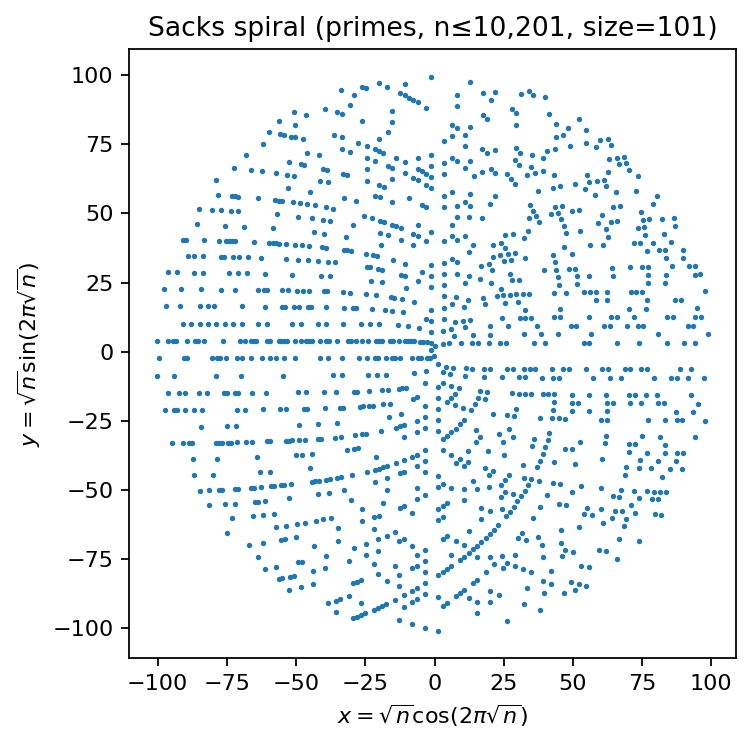
size 101: 10,201 numbers and 1,252 primes

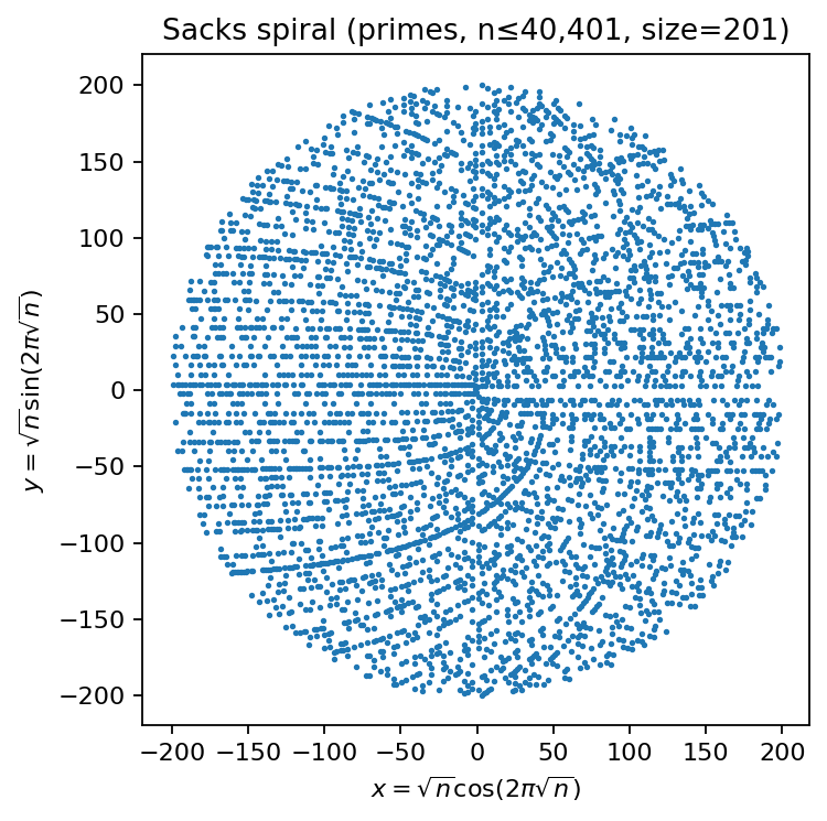
size 201: 40,401 numbers and 4,236 primes

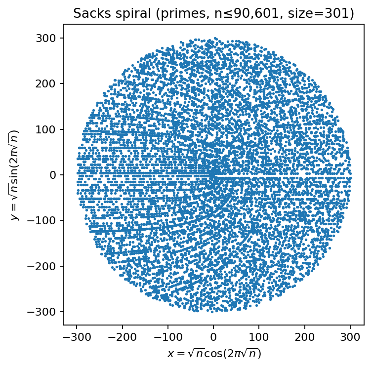
size 301: 90,601 numbers and 8,769 primes

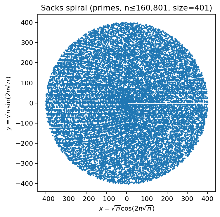
size 401: 160,801 numbers and 14,752 primes

size 999: 998,001 numbers and 78,359 primes

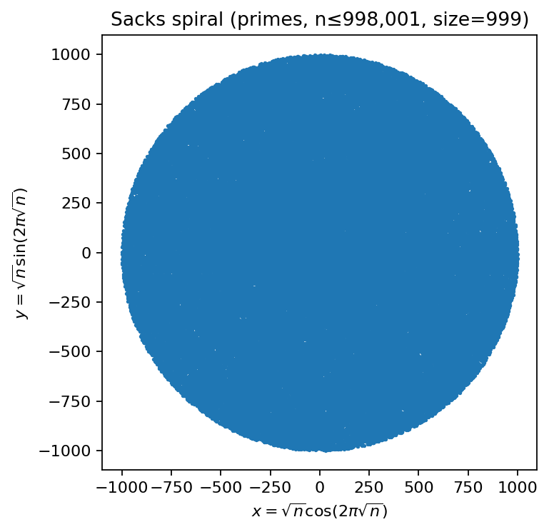
Prime counts shown are \(\pi(\text{size}^2)\), i.e., the number of primes \(\le \text{size}^2\).

Tags: number-theory, quantitative-exploration, visualization
See: Valid Tags.

Highlights

• Places integers on a spiral using polar coordinates \(r=\sqrt{n}\) and \(\theta = 2\pi\sqrt{n}\).

• Parameterizable run: vary --size from the command line (default: 301).

• Writes reproducible artifacts (params.json, report.md, and figures) into out/e125/.

Goal

Render the Sacks spiral and highlight primes as a point cloud to reveal spiral-aligned structure, then compare how the apparent density and “spiral fragments” change as size increases.

Background (quick refresher)

What is the Sacks spiral?

In the Sacks spiral, each integer \(n\) is mapped to polar coordinates

\[r_n = \sqrt{n},\qquad \theta_n = 2\pi\sqrt{n},\]

and plotted as \((x,y) = (r\cos\theta,\ r\sin\theta)\). Highlighting primes yields striking spiral fragments and density variations. See [Brockmann, 2019].

Optional background pages

• Prime numbers refresher

Research question

How does the visual “prime spiral density” change as size increases (i.e., as we include integers up to \(\text{size}^2\)), and which spiral-aligned structures persist across scales?

Why this qualifies as a mathematical experiment

• Finite procedure: compute primes up to \(\text{size}^2\) and apply a deterministic mapping \(n\mapsto(x,y)\).

• Observable(s): spiral fragments, density contrasts, and how visibility changes with size.

• Parameter space: size (and, if you extend it, marker size / rendering choices).

• Outcome: figures and a short report capturing the key observation and caveats.

• Reproducibility: outputs saved to out/e125/ with a parameter snapshot.

Experiment design

• Computation: for integers \(1,\dots,\text{size}^2\), compute a prime mask; map prime indices to \((x,y)\) via the Sacks rule.

• Coordinates: Cartesian coordinates \((x,y)\) are computed from \(r=\sqrt{n}\) and \(\theta=2\pi\sqrt{n}\) via \((x,y)=(r\cos\theta,\ r\sin\theta)\).

• Prime classification: primes are computed deterministically up to \(\text{size}^2\) (sieve).

• Outputs: one or more scatter plots of prime points (composites omitted).

• Artifacts written:

  • figures/fig_01_sacks_spiral*.png (main figure) and figures/e125_hero_<size>.png (published hero)

  • params.json

  • report.md

Axis scaling note

The run includes integers \(n\le \text{size}^2\). With the Sacks choice \(r=\sqrt{n}\), the maximal radius shown is

\[r_{\max}=\sqrt{\text{size}^2}=\text{size},\]

, so the plot naturally fits inside a disk of radius about size.

How to run

make run EXP=e125

Override the experiment size:

make run EXP=e125 ARGS="--size 501"

Direct invocation (always works):

uv run --extra dev python -m mathxlab.experiments.e125 --out out/e125 --size 501

Notes / pitfalls

• Scatter plots are sensitive to marker size and resolution: the same data can look different depending on rendering.

• Larger size means more numbers (\(\text{size}^2\)) and a longer run time.

• “Looks-true” trap: a visually strong spiral does not by itself imply a theorem about primes.

Extensions

• Add a faint background of composite points (with transparency) to compare prime vs. composite geometry.

• Plot multiple sizes on identical axes to compare density and visible spiral fragments.

• Add simple quantitative summaries (e.g., radial density bins for primes vs. all numbers).

Published run snapshot

If this experiment is included in the docs gallery, include the published snapshot (report + params).

Reproduce:

make run EXP=e125

Parameters

• size: 301 (odd); visualizes integers 1..90601.

Notes

• Construction: r = sqrt(n), θ = 2π sqrt(n) so squares align on a ray.

• Prime-rich curves correspond to quadratic polynomials under this embedding.

• This experiment is deterministic; seed does not change the output.

params.json (snapshot)

{
  "size": 301
}

References

• Exposition connecting multiple prime visualizations (includes Sacks spiral): [Brockmann, 2019].

• Recreational-math context and “pattern traps”: [Gardner, 1983], [Hoffman, 1989].

See also References.

Related experiments

• E024: Ulam spiral structure (Ulam spiral structure)

• E124: Klauber triangle structure (Klauber triangle structure)

• E126: Hexagonal number spiral structure (Hexagonal number spiral structure)

• E127: Quadratic prime-run atlas (n^2 + a n + b) (Quadratic prime-run atlas (\(n^2 + a n + b\)))

• E128: Quadratic modular obstructions (Euler-type) (Quadratic modular obstructions (Euler-type))

• E129: Euler lucky constants for n^2 + n + b (Euler lucky constants for \(n^2 + n + b\))

Parameters (example)

• size: 301 (implied total integers: 1..90,601)

Recommended size range

The Sacks spiral run includes integers \(1,\dots,\text{size}^2\), so runtime and memory scale roughly with \(\text{size}^2\) (prime classification dominates).

A practical range that works well for most runs:

• Minimum (still meaningful): size = 101

• Default / recommended: size = 301

• Comfortable upper range on typical laptops (varies): size = 999

• Above ~size = 1501: expect noticeably higher runtime (and potentially memory pressure), depending on the machine and the primality implementation.

Rule of thumb: start with 301, then try 501, 701, 901. Increase further only if runtime remains acceptable.

Summary

We compute primes among the first 90,601 positive integers and plot prime indices using the Sacks polar mapping. Even at this moderate scale, visible spiral-aligned prime fragments emerge, with noticeable density variation across radii.

Key observations

• Prime points form dense spiral segments rather than appearing uniformly “random” in the plane.

• The visibility of segments depends strongly on marker size and figure resolution.

Interpretation

The Sacks mapping is a deterministic geometric transform of the integer line. It tends to visually emphasize arithmetic structure (including sequences with prime-rich behavior), making it a useful exploratory visualization tool — but not a proof technique.

Caveats

• Rendering matters: marker size, DPI, and axis limits can change perceived structure.

• Finite window: patterns can strengthen or weaken as size changes.

• Without quantitative overlays, conclusions remain qualitative.