E001: Taylor Error Landscapes
Tags: analysis, quantitative-exploration, visualization, numerics, taylor
See: Valid Tags.
Goal
Build intuition for Taylor truncation error by visualizing the absolute error landscape \(|\sin(x) - T_n(x; x_0)|\) over a domain while varying:
the polynomial degree \(n\),
the expansion center \(x_0\).
Background (quick refresher)
If you want a short mathematical recap first, read: Taylor series refresher.
Research question
How does the approximation error of Taylor polynomials for \(\sin(x)\) depend on the polynomial degree \(n\) and the expansion center \(x_0\), over a fixed domain of \(x\)?
Concretely: for a chosen grid of \((n, x_0)\), what does the error landscape \(E_{n,x_0}(x)=|\sin(x)-T_n(x;x_0)|\) look like, and where do numerical artifacts start to dominate the truncation error?
Why this qualifies as a mathematical experiment
This page is not just a worked example or a derivation — it is an experiment in the sense of experimental mathematics: a finite, reproducible procedure that produces evidence about how a mathematical object behaves.
For E001, the object is the family of Taylor polynomials \(T_n(x; x_0)\) for \(\sin(x)\), and the observable is the error function \(E_{n,x_0}(x) = |\sin(x) - T_n(x; x_0)|\). The experiment qualifies because it:
Explores a parameter space: it varies degree \(n\) and center \(x_0\) and inspects how the entire error landscape changes.
Generates testable conjectures: e.g. “there is a widening low-error region around \(x_0\) as \(n\) increases” and “improvement is not uniform across a fixed interval”.
Searches for failure modes / edge cases: large \(|x-x_0|\), high degrees, and wide domains can expose numerical artifacts that look like truncation error but are actually floating-point limitations.
Produces artifacts that can be checked independently: plots and parameter snapshots make it easy to compare runs, reproduce the same conditions, and verify that an observed pattern is not accidental.
The goal is to turn “Taylor series should be good near \(x_0\)” into structured evidence about where and how the approximation is good (or bad), which then informs what one would try to prove or bound formally.
How does the truncation error \(|\sin(x) - T_n(x; x_0)|\) behave as we move away from the center \(x_0\)?
How many terms are needed to achieve a specific precision (e.g., \(10^{-6}\)) over a fixed interval?
Does increasing the degree \(n\) always improve the result everywhere in the domain?
Experiment design
Target function: \(\sin(x)\)
Evaluation: \(x \in [-2\pi, 2\pi]\) (default)
Parameters:
degrees: \(\{1, 3, 5, 7, 9\}\)centers: \(\{0, \pi/2, \pi\}\)
Outputs:
Plot of \(f(x)\) vs. \(T_n(x)\)
Semi-log plot of \(|f(x) - T_n(x)|\)
How to run
make run EXP=e001 ARGS="--seed 1"
Artifacts are written under out/e001/ (figures, parameters, and a short report.md).
What to expect
Qualitatively (and this is what the plots should confirm):
near \(x_0\), the higher degree reduces the error quickly,
away from \(x_0\), the approximation can degrade even for higher degrees,
changing \(x_0\) shifts the “low-error region”.
Results
After running the experiment, include (or regenerate) the figures in the documentation.
The canonical output location is out/e001/. For publishing, copy one representative “hero” image into
docs/_static/experiments/ (see “Gallery images” below).
Notes / pitfalls
Use log-scale for absolute error plots to see the full dynamic range.
Be careful interpreting relative error near zeros of \(\sin(x)\).
Huge domains and high degrees can expose floating-point artifacts that are not truncation error.
Extensions
Alternative functions: Repeat the experiment for \(exp(x)\) or \(1/(1-x)\).
Relative error: Plot \(|(f-T_n)/f|\) instead of absolute error.
Automatic degree selection: Find the minimal \(n\) such that error \(< \epsilon\) on a given interval.
Gallery images (recommended)
To keep the experiment gallery attractive and stable:
run the experiment locally,
pick one representative output figure,
copy it into the repo under:
docs/_static/experiments/e001_hero.png
This allows the docs to show thumbnails without depending on generated out/ artifacts.
Published run snapshot
If this experiment is included in the docs gallery, include the published snapshot (report + params).
Reproduce:
make run EXP=e001_taylor_error_landscapes
Seed: 1
Parameters
Domain:
[x_min, x_max] = [-6.0, 6.0]num_points:
4000degrees:
1, 3, 5, 9, 15centers:
0, 1, 2
What this run produces
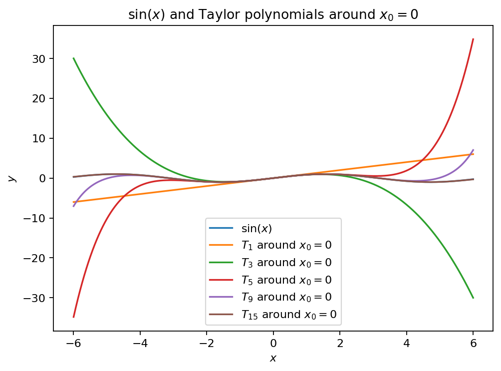
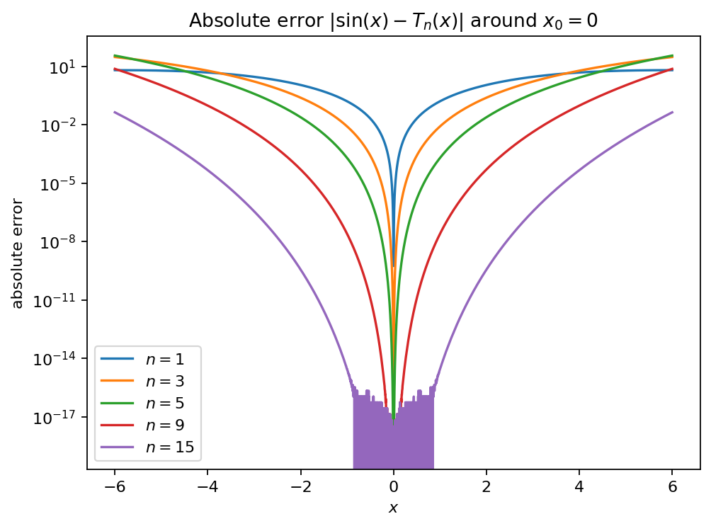
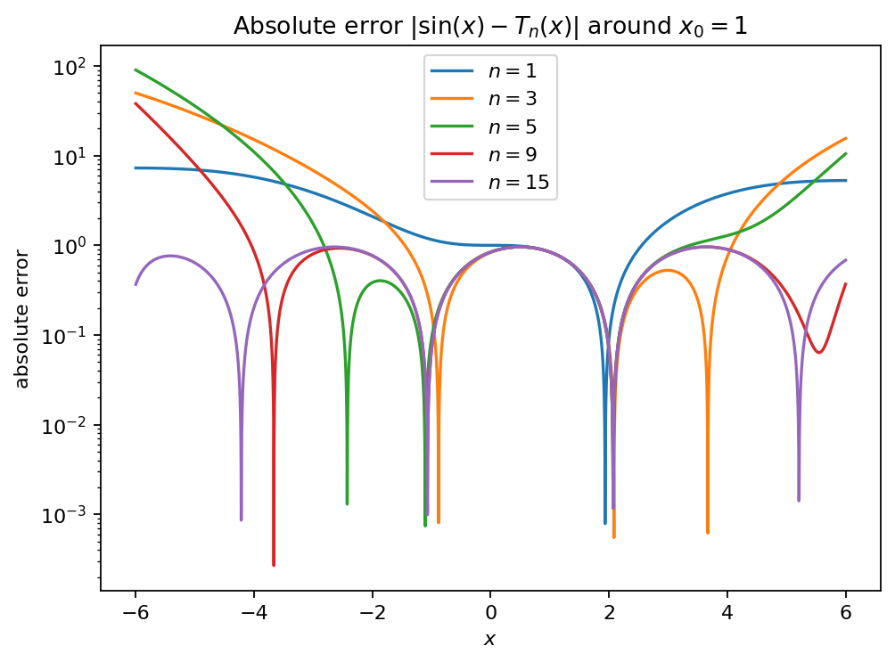
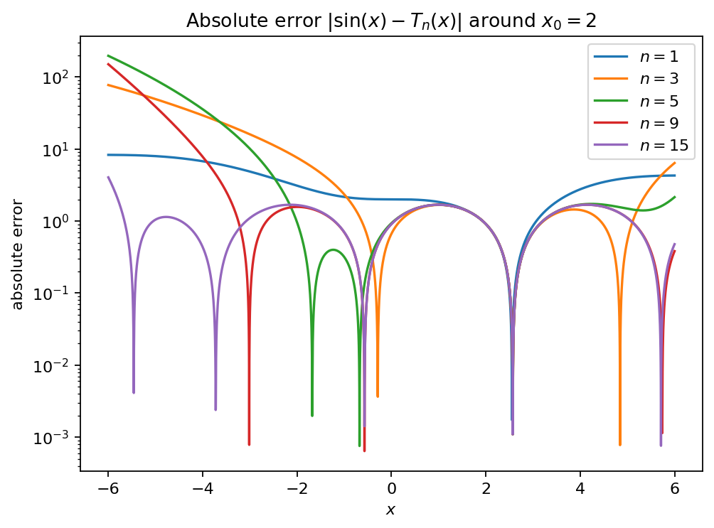
figures/fig_01_sin_and_taylor_center_*.png— overlay of sin(x) and Taylor polynomials for one centerfigures/fig_02_error_landscape_center_*.png— absolute error curves for each center, overlaid by degree
Notes
Taylor approximations are local: accuracy is highest near the expansion center and generally degrades away from it.
If you increase degrees or the domain size, floating-point roundoff may become visible.
params.json (snapshot)
{
  "centers": [
    0.0,
    1.0,
    2.0
  ],
  "degrees": [
    1,
    3,
    5,
    9,
    15
  ],
  "num_points": 4000,
  "x_max": 6.0,
  "x_min": -6.0
}
References
See References.
[Bailey and Borwein, 2005, Borwein, 2005, Borwein and Bailey, 2008]